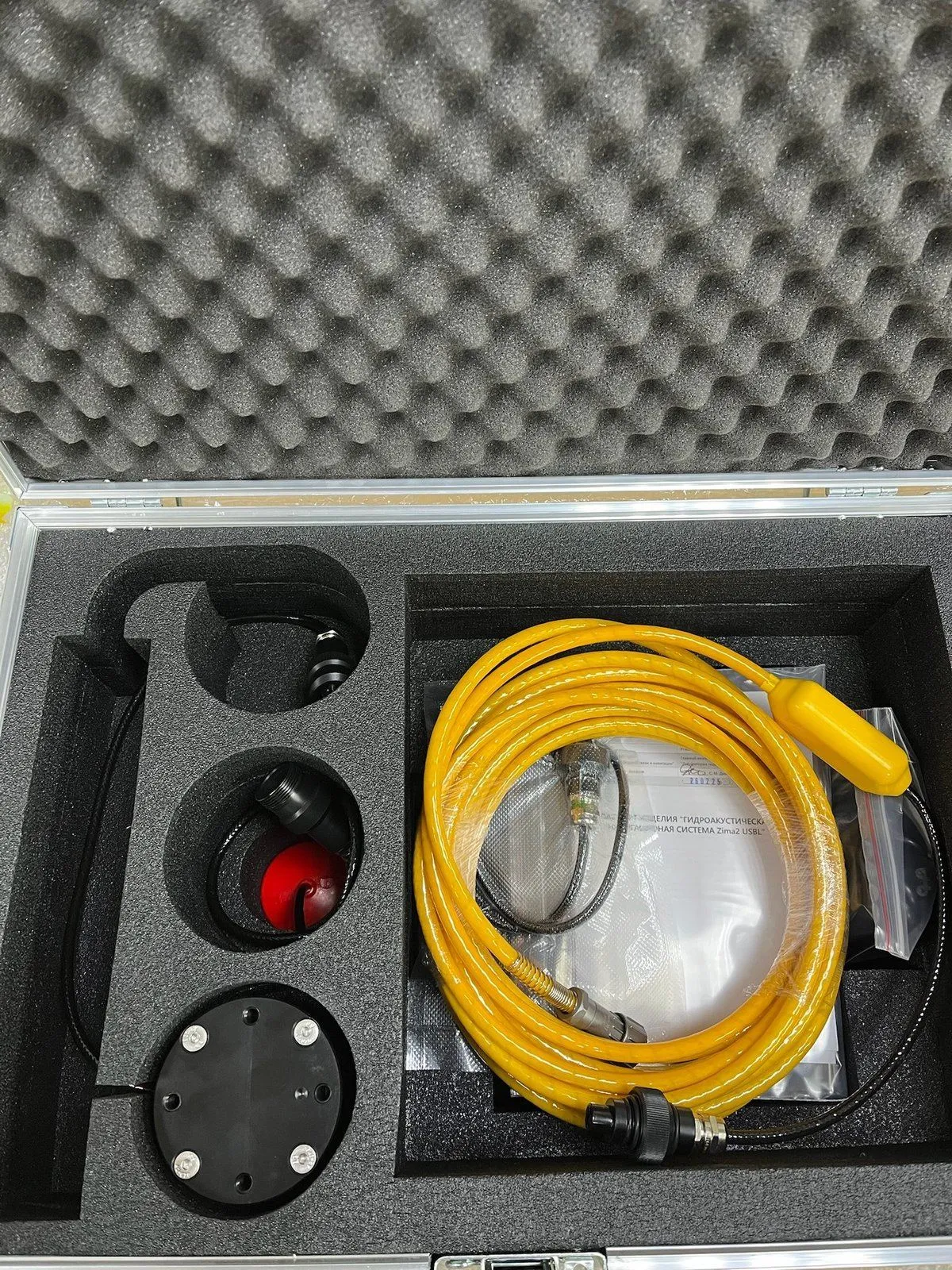
Greetings, dear colleagues! Our “underwater GPS” recently turned three years old. Over that time the system has gone into serial production, we have brought several more systems and devices to market, but the whole time we've been haunted by one idea: bringing hydroacoustics to the masses, making it accessible to amateurs, hobbyist builders, citizen-science folks, and anyone else who's curious.
So today, to mark our modest anniversary, we'll walk you through, in plain terms, how to determine an underwater object's geographic position using just two transceivers: with source code, fun pictures, graphs, and experimental results.
WARNING: this article contains trace amounts of math!
For those who don't understand what's going on but wouldn't mind digging in, we suggest checking out our previous articles on hydroacoustics and underwater navigation:
A video transmission session through water via sound, with the trick exposed
Underwater GPS from scratch in a year
Underwater GPS: the sequel
On the effect of cyanobacteria on presidential speech function
Underwater navigation: bearing or no bearing, you're doomed to succeed
As well as an excellent overview article on hydroacoustics
Preliminaries
Underwater, radio waves don't travel any meaningful distance, and — let's be honest — any decent wireless communication and navigation down there is only possible using acoustics.
Today there are three main working types of navigation systems:
- ultra-short-baseline (USBL) — based on determining the angle of arrival of the beacon's signal and measuring the range (either by the request-response method or with synchronized clocks). The angle of arrival is determined with an antenna array. The sought position is found from the angle and the range (a direct geodetic problem). Our Zima, for instance, is a USBL system;
- long-baseline (LBL) — where the arrival times of a signal are measured either at several receivers, or from several transmitters (this is exactly how our underwater GPS works) with a known position. You can either measure distances by the request-response method (a ranging approach) or measure the differences in signal arrival times (a hyperbolic/time-difference approach) — this is how GPS and GLONASS work, for example. A long baseline can be floating (like our RedWave) or seabed-mounted;
- short-baseline (SBL) — essentially the same as long-baseline systems, except that all the base's reference elements sit on a single platform — a vessel, for example.
As mentioned above, a long baseline can work on the “request-response” principle, in which case you need to solve the problem of the intersection of N spheres — or circles, if the target's depth is known.
Or the base can work the same way as GPS and GLONASS; such systems are also called hyperbolic, and here's why: if the target periodically emits a navigation signal and the clocks of all the receivers (base elements) are synchronized, the distance cannot be measured directly — you can only tell which base element the source is closer to or farther from. In other words, all you have are differences in distance. And as we know from school:
“A hyperbola can be defined as the locus of points for which the absolute value of the difference of the distances to two given points, called foci, is constant.”
In other words, if an underwater object emits a signal and we pick it up on two receivers with synchronized clocks, we can say that our object lies on a hyperboloid (or on a hyperbola, if it also sent us its depth). More receivers mean more hyperbolas, and more hyperbolas mean higher positioning accuracy.
And if it's not the underwater object that transmits, but the base elements instead, then the underwater object, knowing its own depth, can determine its own position; moreover, in this case it doesn't interfere with anyone else, and there can be as many such objects as you like — they're all just listeners. That's how GPS/GLONASS and our own RedWave work.
But we promised navigation with two transceivers, one of which is the very one whose position we need to find.
Let's dig in
The distance between two points A(xa,ya,za) and B(xb,yb,zb) in three-dimensional space is given by a simple formula:

Suppose we have N base stations. Assume their coordinates are known, and that we have measured the distances dbn from each base station Bn(xbn,ybn,zbn) to the target T. For clarity: T stands for target, and B for base.
So for any point M(x,y,z), we can write an expression that shows how well that point fits our experimental measurements. In effect, this is the sum of the differences between the distance from point M to the corresponding base station and the measured distance. We square each of these differences:

In short, this leads to the least-squares method, and ideally the coordinates of the target point should minimize the error function ε.
If instead we're using the time-difference-of-arrival method, which is what this article will cover, and each base station gives us not a measured distance dbn but a signal arrival time tOA, then the error function will contain not distances but their differences. The only extra wrinkle is that you need to go through the relevant pairs of base stations — for example, for station n and station n+1:
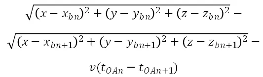
Here v is the speed of sound, which, as we know, is not constant — it depends heavily on the density of the medium, i.e., on temperature, salinity, and pressure. If you want to compute everything precisely, you either have to measure it directly or calculate it (that deserves its own separate article).
Note that in modern hydroacoustic navigation systems, the depth of positioned objects is measured directly, with fairly high accuracy (0.5–2 cm), so it makes sense to reduce the problem to a planar one.
We could just say: now solve this with any optimization method, and call it a day. But firstly, it's not that simple, and secondly, it's not that complicated.
Let's start with the difficulties
The thing is, a lot depends on how the base stations are arranged relative to each other (which you can influence to some extent, say, through administrative methods =)) and on the position of the target relative to the base elements (which is much harder to influence — in a wide range of tasks, the target's initial position is only very roughly known, so it's nearly impossible to set up the base advantageously in advance).
In practice, we're most likely to end up with a situation like this:
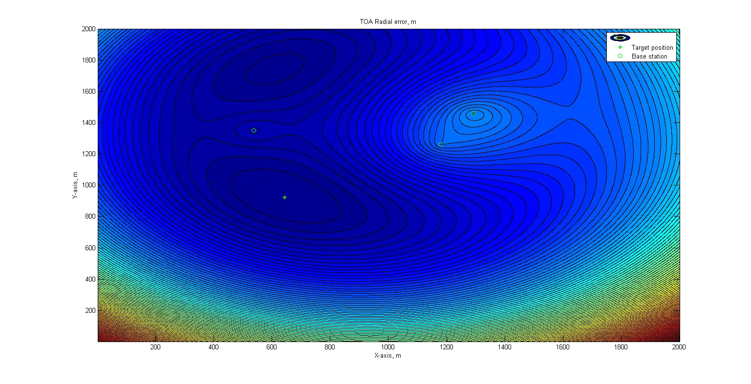
Figure 1 — Error surface for a three-element base. The target is outside the base. A false minimum is present
Green circles mark the positions of the base stations, and the star marks the target's true position. The color of each point shows the value of the residual function (ε) at that point. As you can see, the surface has two basins, and it's very easy for a minimum search to fall into the wrong one. In practice, things are even worse: given the scale, the object's actual position, and the typical speed of such objects, it will stay in roughly the same spot for quite a while, the shape of the error surface will remain the same, and there's a very high chance of getting incorrect position data for an extended period.
The animation below illustrates a similar situation — whether the search starts from the midpoint between the base stations or from the nearest station, it converges to the false minimum:
Figure 2 — The search falling into the false minimum when starting from the base's midpoint. A three-element base
The search here is implemented using the Nelder-Mead algorithm, also known as the simplex method. This is, for instance, exactly what MATLAB's fminsearch function uses.
It requires no derivative calculations, is very visual, intuitive, and simple to implement.
Figure 3 — The search falling into the false minimum when starting from the nearest base element. A three-element base
Knowledgeable readers might object that nobody places base stations in a straight line — but firstly, sometimes people actually do, and secondly, it's exaggerated here purely for a clearer demonstration.
“The defeat was total. There was no way to think of anything.” — A. and B. Strugatsky, “The Doomed City”
So what can be done about this?
Logic suggests using one of the global optimization methods — simulated annealing or something similar. However, another, more productive approach is to make fuller use of prior information when choosing the starting point for the search.
After all, we know for a fact that the target point lies (with some approximation) on circles centered on the base stations, with radii equal to the measured ranges!
We're also confident that in hydroacoustics, the range-measurement error grows together with the range itself: sound doesn't propagate linearly.
So we can try choosing the starting point for the minimum search around (literally, on the circle of) the nearest beacon, on the assumption that the range to it was measured with the highest accuracy, guided by that same residual function ε.
In this case, the candidate points' coordinates are formed using the following simple formulas:
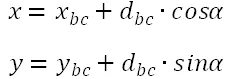
xbc and ybc are the coordinates of the nearest (c for closest) base station, and dbc is the distance from it to the target. a is the argument (angle). If you now search for the minimum of ε by varying a from 0 to 360 degrees in, say, 10-degree steps, and then search again near that value with the step reduced to 1 degree and the search range narrowed to 20 (±10) degrees, you can get a very good initial approximation that, in nearly every case, lands almost exactly on the target right away!
In the pictures below, the brute-force method valiantly landed in the false minimum after 30 iterations, producing a completely wrong solution, while the method with preliminary one-dimensional minimization hit the target almost immediately, converging to within ~25 centimeters of the true position in 6 iterations, at a distance of ~400 meters to the nearest base station.
Figure 4 — The search falling into the false minimum
Figure 5 — Finding the correct solution when starting from the point obtained by preliminary one-dimensional minimization
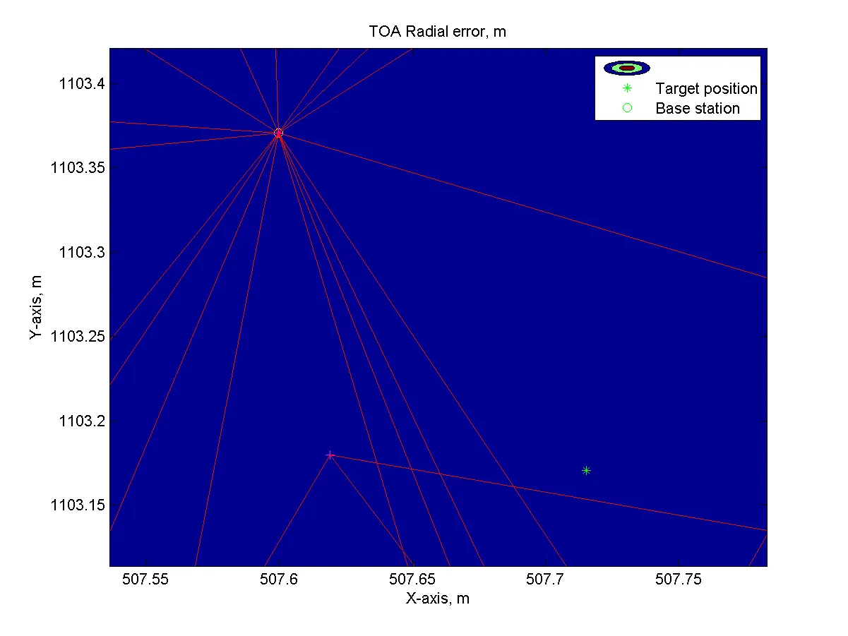
Figure 6 — A zoomed-in area around the resulting solution. The yellow circle is the computed solution, the green star is the object's true position
In the example above, even the very first iteration after the preliminary choice of the starting search position gave a solution within 20 meters of the actual position (on a field of ~600×600 meters).
At this point we've worked out the ranging approach. With the time-difference approach the situation is a bit trickier: there are no such clear landmarks for choosing a starting point (a circle is a nice shape because it's closed, while a hyperbola is awkward because it runs off to infinity).
Let's get back to the promised “underwater GPS” with two transceivers. In a sense, we were, of course, being a bit sneaky: you won't get a full-fledged underwater GPS like the one from our first article, but if you don't have the money for the “proper” device, and you can live with a few limitations and accept that the method only applies to a certain range of tasks, then there's still something you can do.
Consider a situation where the target object is stationary (or moving negligibly slowly). In such cases, instead of several base stations you can actually use just one, but a moving one: this approach is called VLBL, or virtual long baseline. If you don't need to record the underwater object's movement track and just need to determine its location, this is exactly what you need.
This kind of task often comes up when deploying seabed equipment by free-dropping it from a vessel. At significant depths, and with currents present, the equipment's actual position on the bottom can differ substantially from the point where it was dropped. That equipment can even be an element of a seabed navigation base itself: to determine the position of an underwater object, you first need to determine the position of an underwater object.
So how might all of this actually work in the real world?
Our experimental setup consists of:
the object we'll be hiding on the bottom of the water body: our RedGTR code modem in a standalone configuration (a modem connected to a sealed battery box). Here it is in the photo:
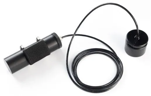
Figure 7 — Responder-beacon with a battery canister
a moving base station built on a cheap Chinese fishing-lure boat from our other article. On board, besides its stock control electronics, it carries a second RedGTR modem, a DORJI 433 MHz radio module with an antenna, a home-built GPS/GLONASS module based on the Quectel L76, and our own board built around an STM32F429 (easily swapped for a NUCLEO-F429ZI or an STM32F4 Discovery), which simply acts as a router: everything from the radio channel goes to the modem over UART and back, and data from the GPS module is likewise pushed out over the radio channel.
Here's what it looks like assembled:
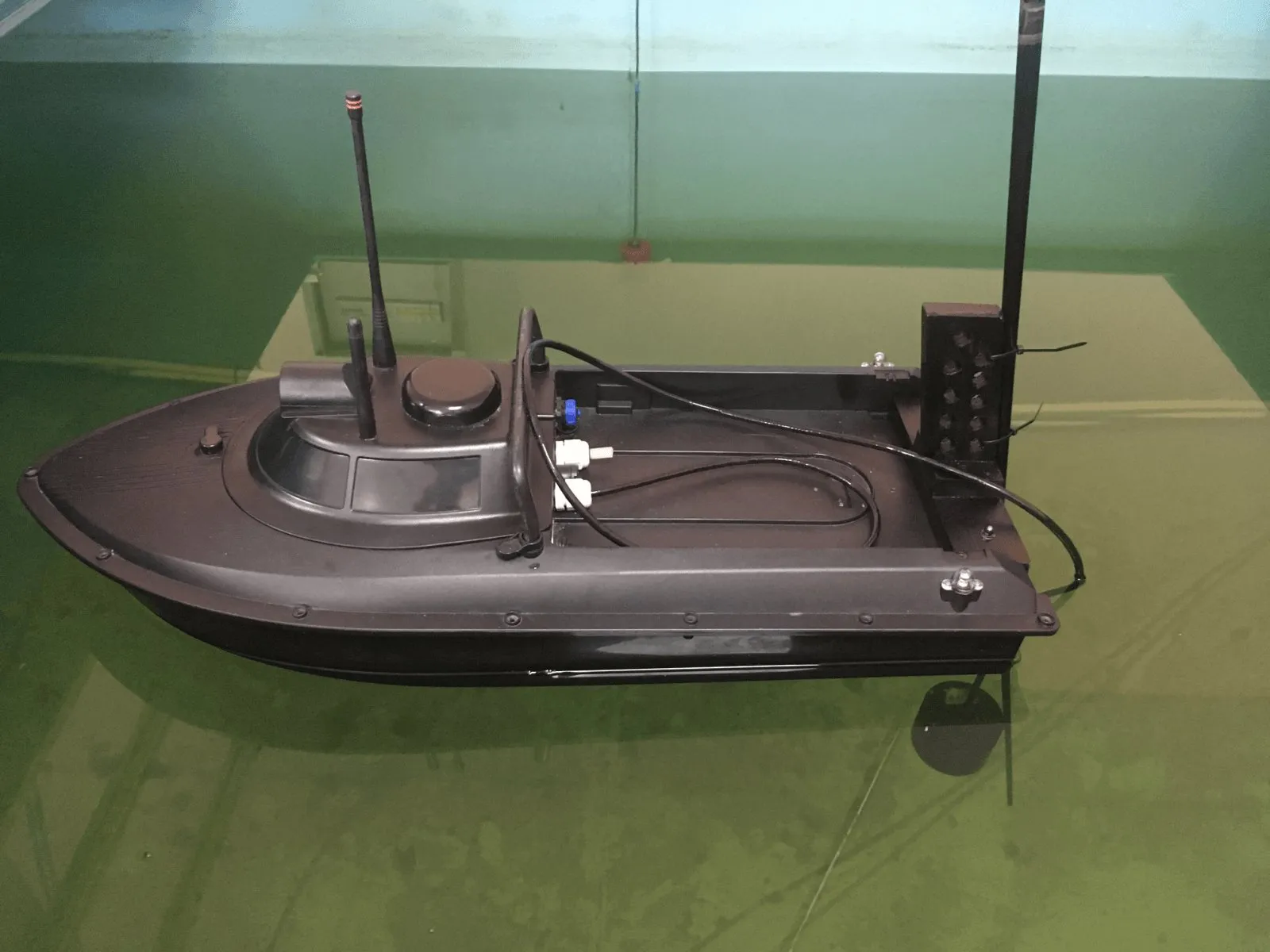
Figure 8 — Photo of the assembled test vessel
This time we improvised a kind of transom out of scrap materials to mount the pole with the modem; our experience with a freely towed navigator had shown this scheme to be flawed, both in terms of controllability and because of the changing relative position between the device and the boat.
Here's what it looks like inside the hull:
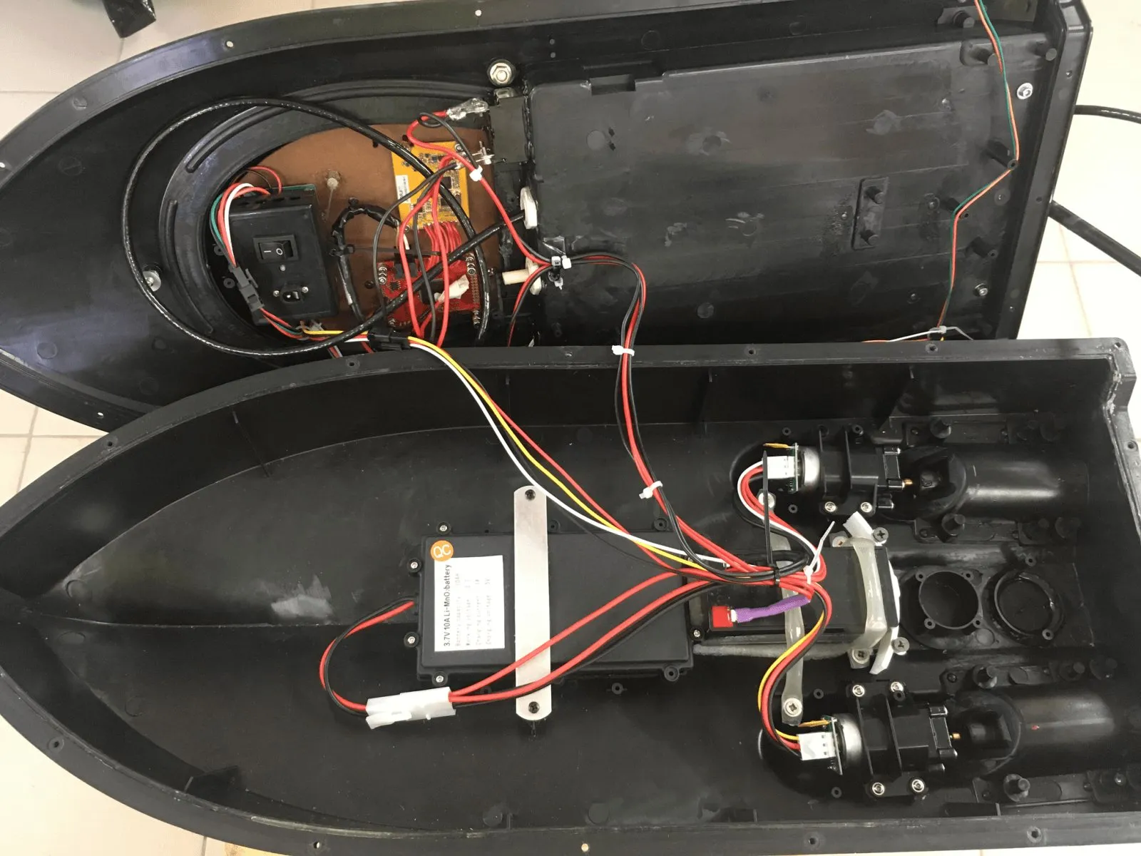
The stock circuitry was left almost entirely unchanged, and all the additional equipment is powered by a separate 1.2 Ah lead-acid battery.
- the operator's console, consisting of a laptop running our software and a matching radio module connected via a USB converter. The software was written, as they say, on the knee, and is only good for a demo, but it already implements the modem interaction protocol, a TOA solver based on the same Nelder-Mead method, base point selection, methods for displaying geographic positions, and the ability to emulate GPS for feeding data into Google Earth or similar programs.
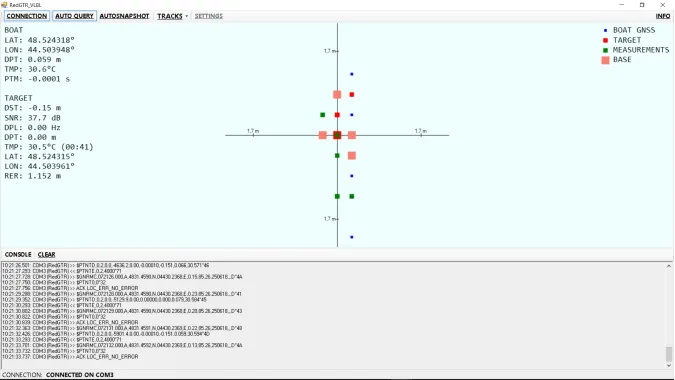
Blue dots are the boat's GPS positions, green dots are the positions where measurements were taken, salmon marks the positions of the virtual base elements, and red marks the computed positions of the responder-beacon.
Who does what?
- the modem we need to locate just sits on the bottom, listening and answering requests;
- the modem on the boat executes the commands it receives over UART — it sends requests and receives responses, reporting them back over UART;
- the STM32F4 board on the boat receives data from the GPS and the modem over UART and forwards it to the radio module over a second UART, and forwards data from the radio module to the modem. There's a small catch related to the radio module — it isn't full-duplex (just like in hydroacoustics =)) — so the board “holds back” the RMC message from the GPS module and only sends it out together with the message from the modem;
- the host software drives the whole process, collects distance-to-target data from various geographic positions, picks the optimal base, and determines the target's location.
A bit more detail
Communication with the modems uses an NMEA-like protocol. For our purposes, only three messages are used:
$PTNTE,targetAddr,requestedCmd,timeoutMs*hh
from the console to the modem. Send the command requestedCmd to the remote node at address targetAddr, with the response timeout set to timeoutMs.
The command can be any one of the approved list:
Command Code Description
CDS_CMD_PING 0 A PING request, to which the remote node replies with PONG
CDS_CMD_PONG 1 Reply to a PING request
CDS_CMD_DPT 2 Command telling the remote node to send its depth
CDS_CMD_TMP 3 Command telling the remote node to send its temperature
CDS_CMD_BAT 4 Command telling the remote node to send its supply voltage
CDS_CMD_USR_0 5 User command 1
CDS_CMD_USR_1 6 User command 2
. . .
CDS_CMD_USR_34 39 User command 34
The modem supports basic functions: ping, sending depth, water temperature, battery charge, and a set of user-defined coded commands.
In response to a TNTE command, the modem immediately replies with an ACK message confirming that the command was accepted, or that it cannot be executed:
$PTNT0,errCode
errCode is 0 if the modem accepted the command, otherwise it's an error code.
If the modem doesn't receive a response from the remote node in time, it reports this with a REM_TIMEOUT message, whose parameter field contains only the remote node's address:
$PTNTB,targetAddr
If the modem receives the response in time, it reports this with a REM_PONGEX command, formatted as follows:
$PTNTD,requestedAddr,requestedCmd,receivedValue_decoded,snrd,dpl,pTime,[dst],[dpt],[tmp]
requestedAddr – the address of the requested node
requestedCmd – the requested command
receivedValue_decoded – the received value
snrd – the signal-to-noise ratio at the receiver output, in dB
dpl – the Doppler shift, in Hz
pTime – the (one-way) signal propagation time, in seconds
dst – the distance to the node, in meters
dpt – the modem's own depth, in meters
tmp – the ambient water temperature, in degrees Celsius
The last three parameters are only sent if the modem has the built-in pressure/temperature sensor option (which is our case).
From the GPS module, we're only interested in the RMC message, from which we get the current geographic position.
The hardest part — transmitting data through water and measuring distance — is handled by the modems, and determining the boat's geographic position is handled by the GPS module. All that's left is the small matter of putting that data to proper use.
All the NMEA message parsing and building is done using the NMEAParser class in the UCNLNMEA library.
The host software running on the laptop periodically sends REM_PINGEX requests to the node at the address configured in the app's settings, doing so as soon as it gets either a REM_TIMEOUT or a REM_PONGEX. Along the way, it records the boat's coordinates and saves the distance and depth data for the remote node together with the boat's coordinates at the moment they were received.
Common sense (and experience) tells us that determining the position of an underwater object takes 3-5 virtual base stations, and, as the pictures above show, they can't just be placed anywhere.
This gives us the following task: as measurements come in, we need to select several of them, in a particular way, to serve as elements of the navigation base.
Here's the approach I propose: choose measurements that form as convex a figure as possible, circumscribed around the assumed location of the target.
To do this, we take some point (at the very start, when we have no idea where the target is, the average of all measurement points will do, and it's later replaced with the first approximation of the target's position), and compute the azimuth (the angle between north and the direction to that point) from it to each measurement point. Then we pick several of them that cover the resulting range of angles as evenly as possible. In the host software, this is done by the List Measurements.GetBase() method;
As data comes in, in the method that parses the REM_PONGEX message, we add the measurements and try to build a navigation base and solve the navigation problem with it. This is handled by the method GeoPoint3DWE LocateLBL_NLM(List base, GeoPoint3DWE prevLocation, double rErrorThreshold, out double stStageRErr, out int itCnt);
It's passed the base itself — the set of measurements we selected for solving the navigation problem — the previous position (if there is one; the target's depth is also passed there), a radial-error threshold, and two diagnostic output parameters: the radial error from the first stage of the solution (one-dimensional optimization) and the number of iterations after which the second-stage solution was obtained.
If we're happy with the resulting solution's radial error, we use that solution as the reference point for building the base.
And so it goes, until we get tired of it, a satisfactory solution is obtained.
As the name suggests, the LocateLBL_NLM method solves the problem using the Nelder-Mead algorithm, first running a one-dimensional optimization if there's no previous solution. In practice you don't have to rely on the previous result at all, and can run the one-dimensional optimization every time — the strategy can vary depending on the specific conditions.
For simplicity, the solution is computed in meters, so before solving, all coordinates are converted to a local coordinate system with its origin at the navigation base's midpoint. After solving, the result is converted back to geographic longitude and latitude (longitude is X, latitude is Y). To convert degrees to meters and back, the Navigation class provides the GetDistance2DDeg and Meters2Deg methods.
But, as we all know, theory without practice is dead, so it's time to move on to the results of our field experiments.
Let's bring the theory to life with a practical check
As is tradition, we ran the trials at the mouth of the Pichuga River. It's a convenient spot, with depths of nearly 30 meters and a fairly challenging underwater terrain.
The responder-beacon is mounted on a special “rig” (the foam floats and the anchor that keep the whole structure upright aren't visible in the frame):
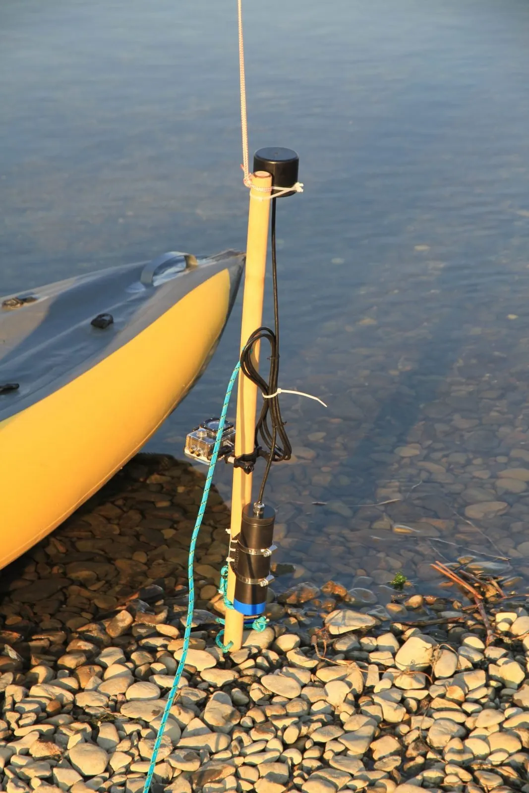
We recorded the beacon's deployment on video; we misjudged the lighting a bit and forgot to bring a flashlight, so the moment it touched the bottom stayed hidden in darkness.
While getting ready for the trials, we gave the little boat a name:
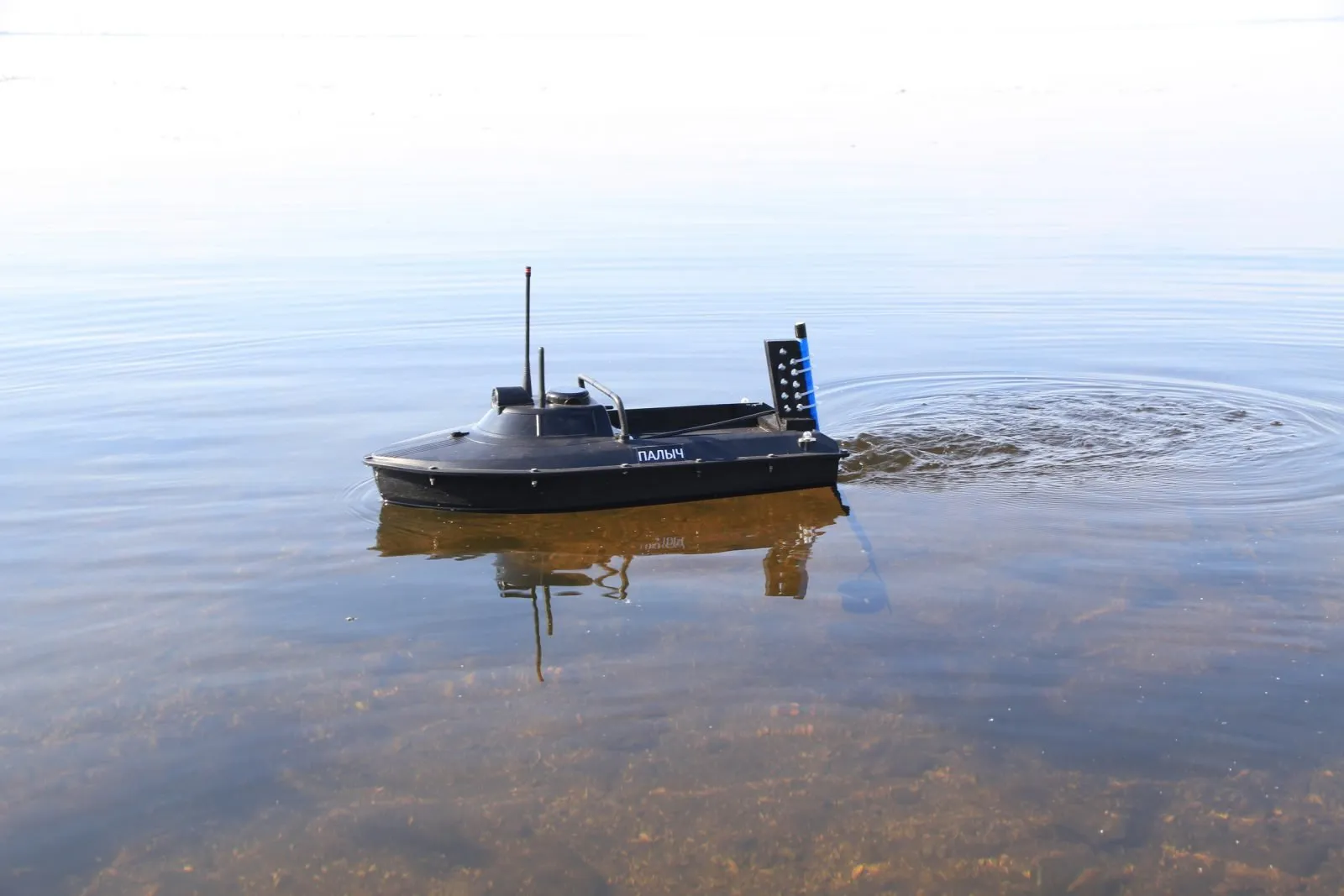
Figure 12 — “Palych” in its natural habitat
A piece of a fishing rod is zip-tied to “Palych's” transom, and the RedGTR modem is mounted on it (so it doesn't dangle or float up).
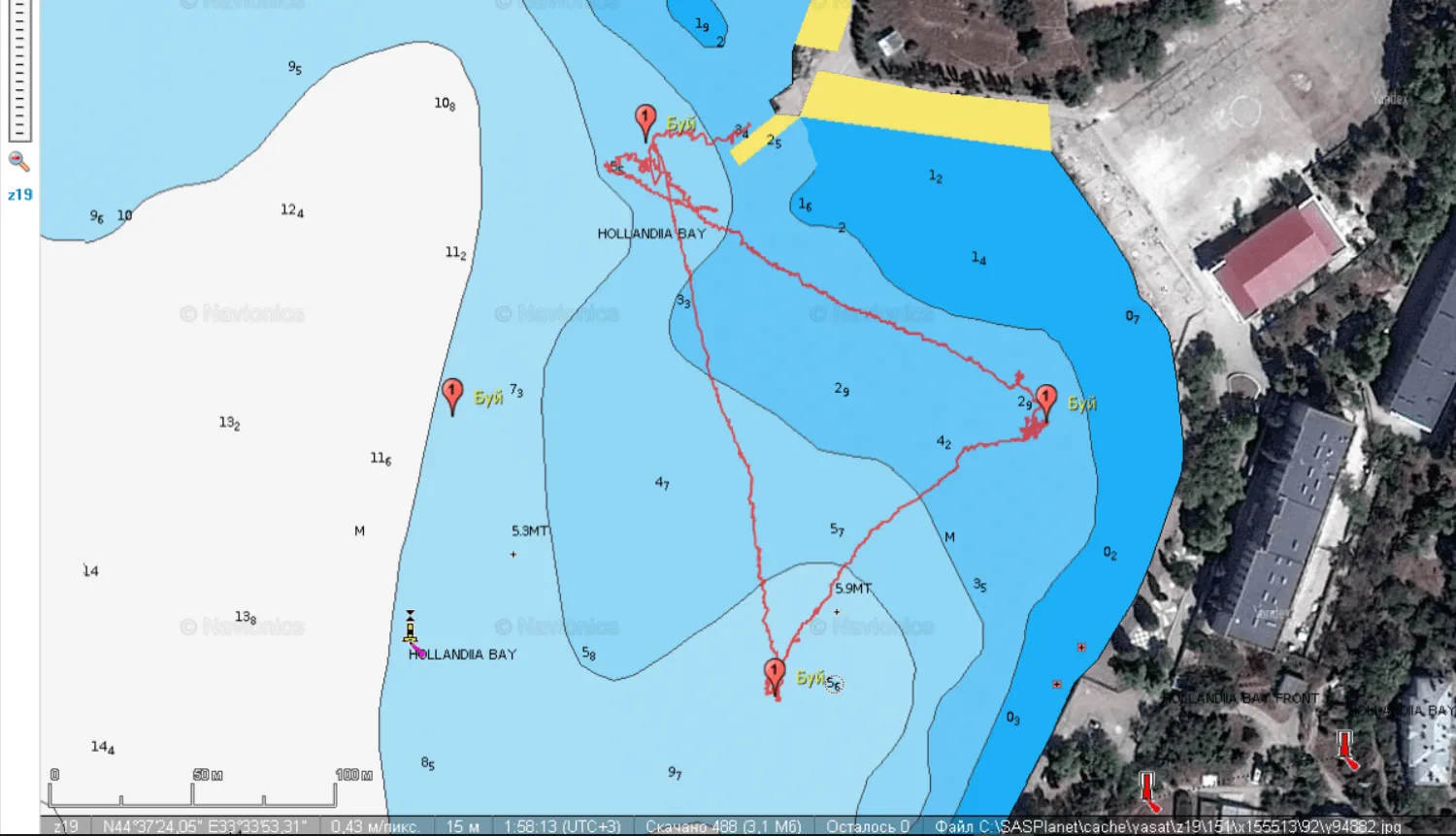
The experiment worked as follows: the responder-beacon is placed on the bottom, with only a small float sticking up above it; “Palych”, remote-controlled from shore, cruises the area in big circles while the host software periodically asks the responder for something, say its depth. All the data is logged, and the screen shows everything as it actually stands. Like this:
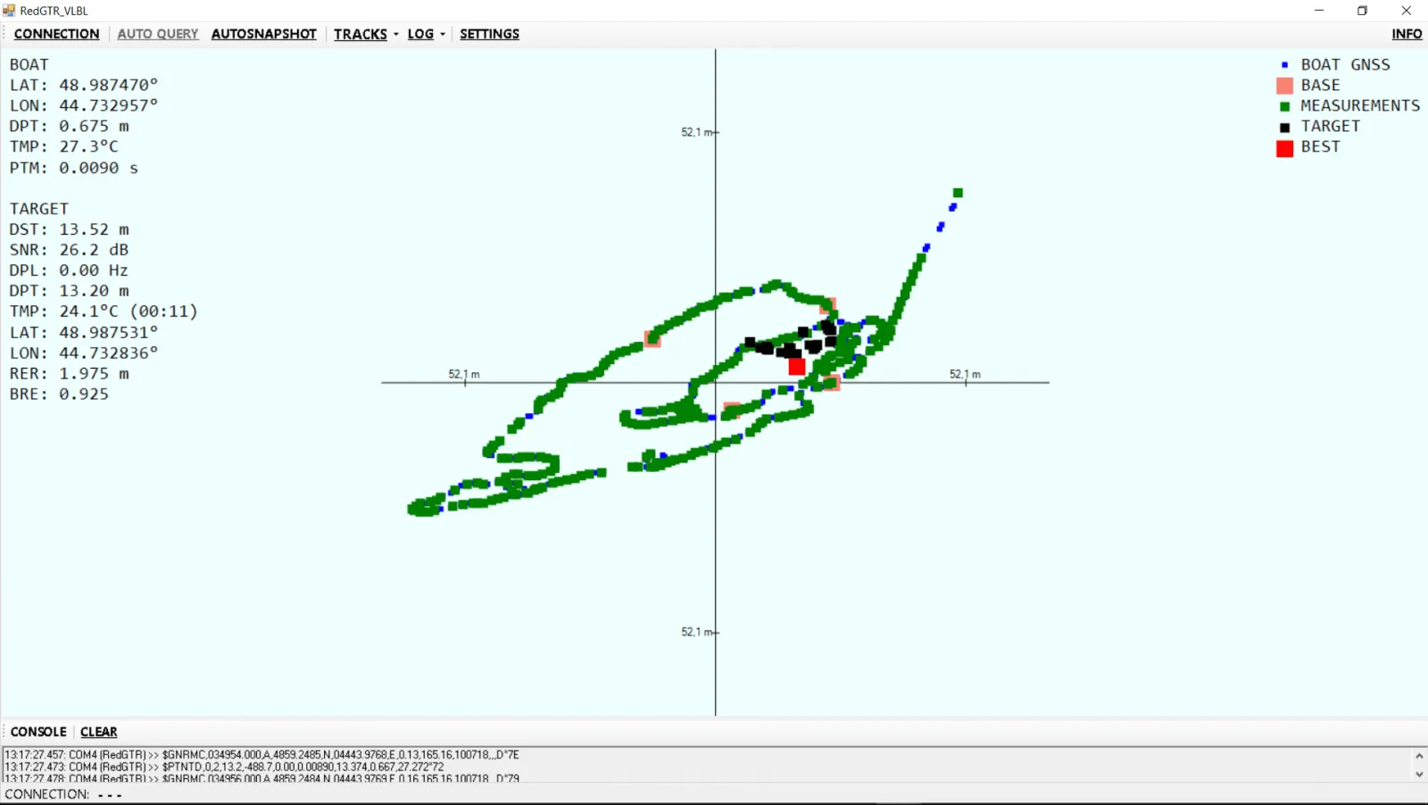
Figure 13 — Screenshot of the host software showing the boat's track and the computed positions of the responder-beacon (red marks the best computed position)
As Figure 13 shows, the beacon was at a depth of 13.2 m, and the water temperature at that depth was 24.1 °C.
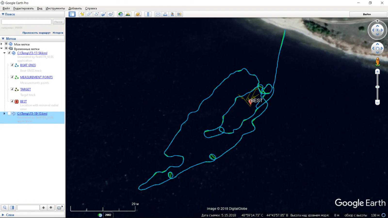
Figure 14 — Importing the resulting tracks into Google Earth
Getting a good result in this case took, at most, about 15 minutes of sailing around.
In the second experiment, the beacon was placed at a depth of 16.5 meters, where it was, predictably, a bit colder — just 22.6 °C.
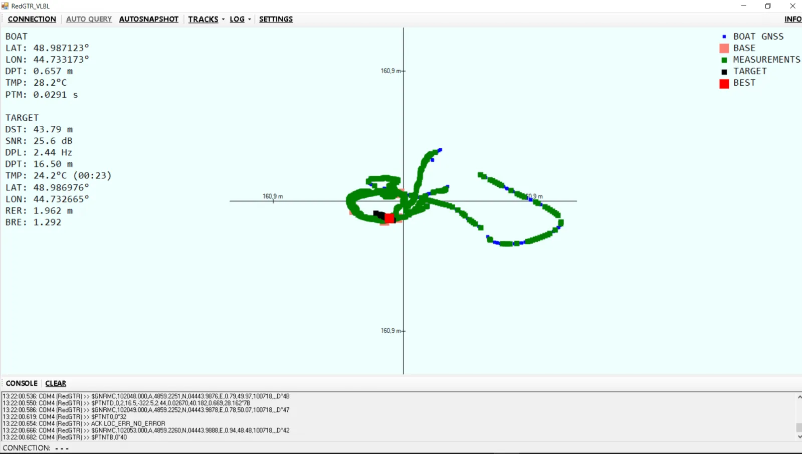
Figure 15 — The responder-beacon position solution from the second experiment, on the host software's screen
We didn't formally assess accuracy in this case, given how short on time we were, and instead settled for the fact that when the boat approached the float (you can see this moment on the first track), its plan-view position matched the best solution exactly, and the range matched the depth (accounting for the depth difference between the responder and the modem mounted on the boat). We recorded the points where the beacons were dropped, and the discrepancy between the computed position and the drop points came out to around 2-3 meters, which further confirms the system works.
All in all, we can say this proof of concept was a success.
Afterword
It's a bit of a shame that the modems used in this experiment, while very cheap by the standards of the global hydroacoustic-communication market, still aren't free.
To give you a sense of world price levels, here's a link to Ms. Benson's excellent thesis; on page 54 of the PDF (page 36 by the document's own numbering) there's a rather interesting little table of prices for various hydroacoustic modems as of 2010 (the table has a small error — the Range for the modem she was developing is given in meters, even though the column header says km).
The good news is that we've developed modems that can do almost all the same things (a bit smaller, shorter range, lower data rate), and, by our estimate, are now priced within reach of well-off enthusiasts.